Histogram Visualization
pyhs3 provides convenient methods to convert data objects into hist.Hist histograms for visualization and analysis using the scikit-hep ecosystem.
Converting Data to Histograms
pyhs3 provides to_hist() methods on several data classes that convert them into hist.Hist objects. These histograms can then be plotted using matplotlib or other visualization tools.
BinnedData to hist
BinnedData represents histogram data with bin contents and optional uncertainties. The to_hist() method creates a hist.Hist object that preserves the binning and uncertainties.
1D Regular Binning
from pyhs3.data import BinnedData
from pyhs3.axes import BinnedAxis

# Create binned data with regular binning
data = BinnedData(
    name="example",
    type="binned",
    contents=[10.0, 20.0, 15.0, 25.0, 18.0],
    axes=[BinnedAxis(name="x", min=0.0, max=5.0, nbins=5)]
)

# Convert to hist and plot
h = data.to_hist()
h.plot(histtype="fill", alpha=0.7, label="Signal")
plt.xlabel("x")
plt.ylabel("Events")
plt.legend()
plt.title("1D Regular Binning")
1D Irregular Binning
from pyhs3.data import BinnedData
from pyhs3.axes import BinnedAxis

# Create binned data with variable-width bins
data = BinnedData(
    name="variable_bins",
    type="binned",
    contents=[5.0, 15.0, 8.0],
    axes=[BinnedAxis(name="pt", edges=[0.0, 10.0, 50.0, 100.0])]
)

# Convert to hist and plot
h = data.to_hist()
h.plot(histtype="step", linewidth=2, label="pT distribution")
plt.xlabel("pT [GeV]")
plt.ylabel("Events")
plt.legend()
plt.title("Variable-Width Bins")
Binned Data with Uncertainties
from pyhs3.data import BinnedData, GaussianUncertainty
from pyhs3.axes import BinnedAxis

# Create binned data with uncertainties
contents = [12.5, 18.3, 15.7, 22.1, 19.4]
sigma = [3.5, 4.3, 4.0, 4.7, 4.4]

data = BinnedData(
    name="with_errors",
    type="binned",
    contents=contents,
    axes=[BinnedAxis(name="mass", min=100.0, max=150.0, nbins=5)],
    uncertainty=GaussianUncertainty(type="gaussian_uncertainty", sigma=sigma)
)

# Convert to hist and plot with error bars
h = data.to_hist()
h.plot(yerr=True, histtype="errorbar", marker="o", label="Data")
plt.xlabel("Mass [GeV]")
plt.ylabel("Events")
plt.legend()
plt.title("Histogram with Uncertainties")
2D Histograms
from pyhs3.data import BinnedData
from pyhs3.axes import BinnedAxis

# Create 2D binned data (3x4 = 12 bins)
contents = [1.0, 2.0, 3.0, 4.0,
            5.0, 6.0, 7.0, 8.0,
            9.0, 10.0, 11.0, 12.0]

data = BinnedData(
    name="2d_hist",
    type="binned",
    contents=contents,
    axes=[
        BinnedAxis(name="x", min=0.0, max=3.0, nbins=3),
        BinnedAxis(name="y", min=0.0, max=4.0, nbins=4),
    ]
)

# Convert to hist and plot as heatmap
h = data.to_hist()
plt.pcolormesh(*h.axes.edges.T, h.values().T, cmap="viridis")
plt.colorbar(label="Events")
plt.xlabel("x")
plt.ylabel("y")
plt.title("2D Histogram")
UnbinnedData to hist
UnbinnedData represents individual data points (events). The to_hist() method bins these entries according to the axis specifications.
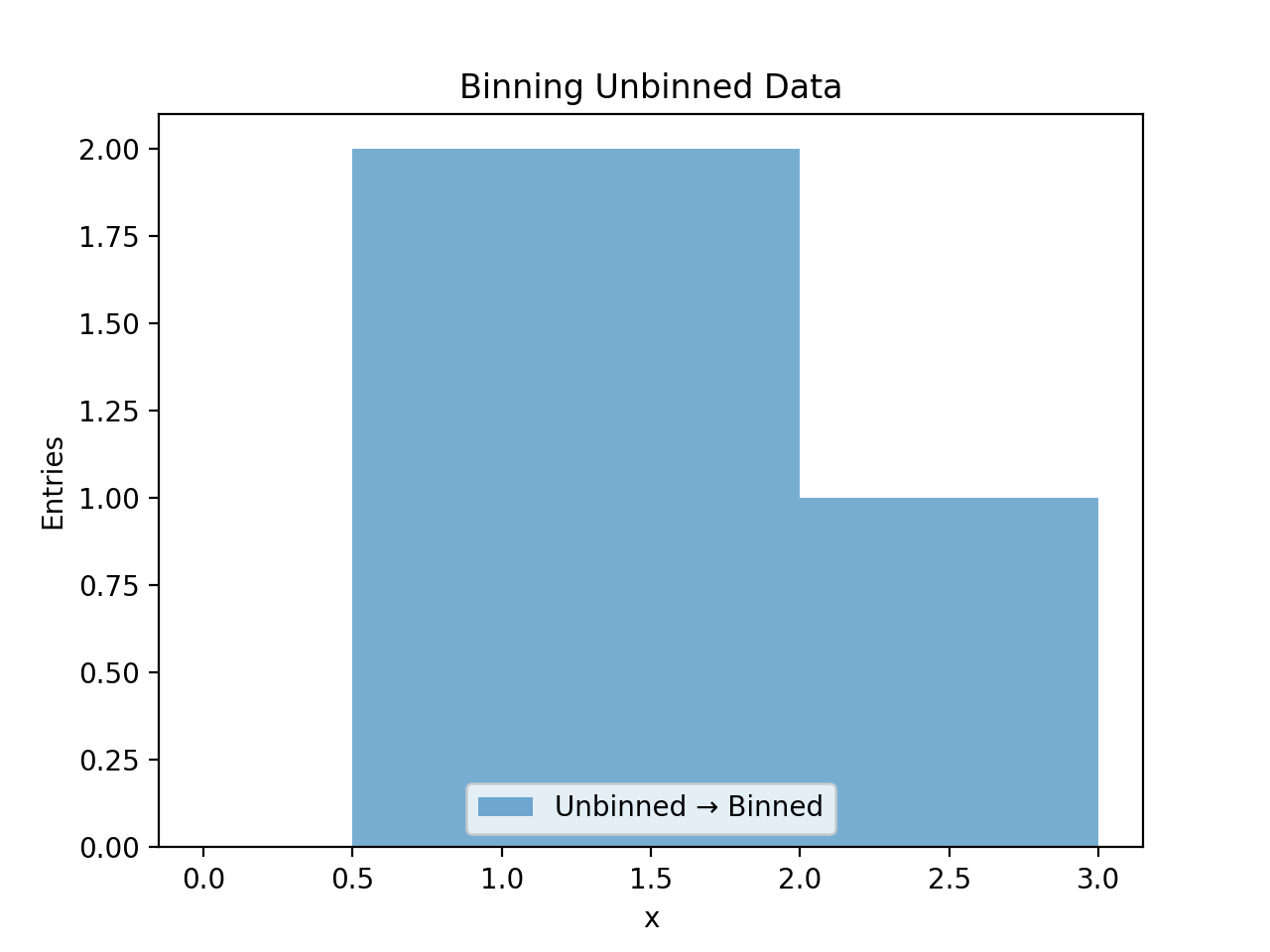
1D Unbinned Data
from pyhs3.data import UnbinnedData
from pyhs3.axes import UnbinnedAxis

# Create unbinned data points
entries = [[0.5], [1.2], [1.8], [2.3], [0.9], [1.5], [2.7], [1.1]]

data = UnbinnedData(
    name="events",
    type="unbinned",
    entries=entries,
    axes=[UnbinnedAxis(name="x", min=0.0, max=3.0)]
)

# Convert to hist by binning the entries
h = data.to_hist(nbins=6)
h.plot(histtype="fill", alpha=0.6, label="Unbinned → Binned")
plt.xlabel("x")
plt.ylabel("Entries")
plt.legend()
plt.title("Binning Unbinned Data")
(Source code, png, hires.png, pdf)

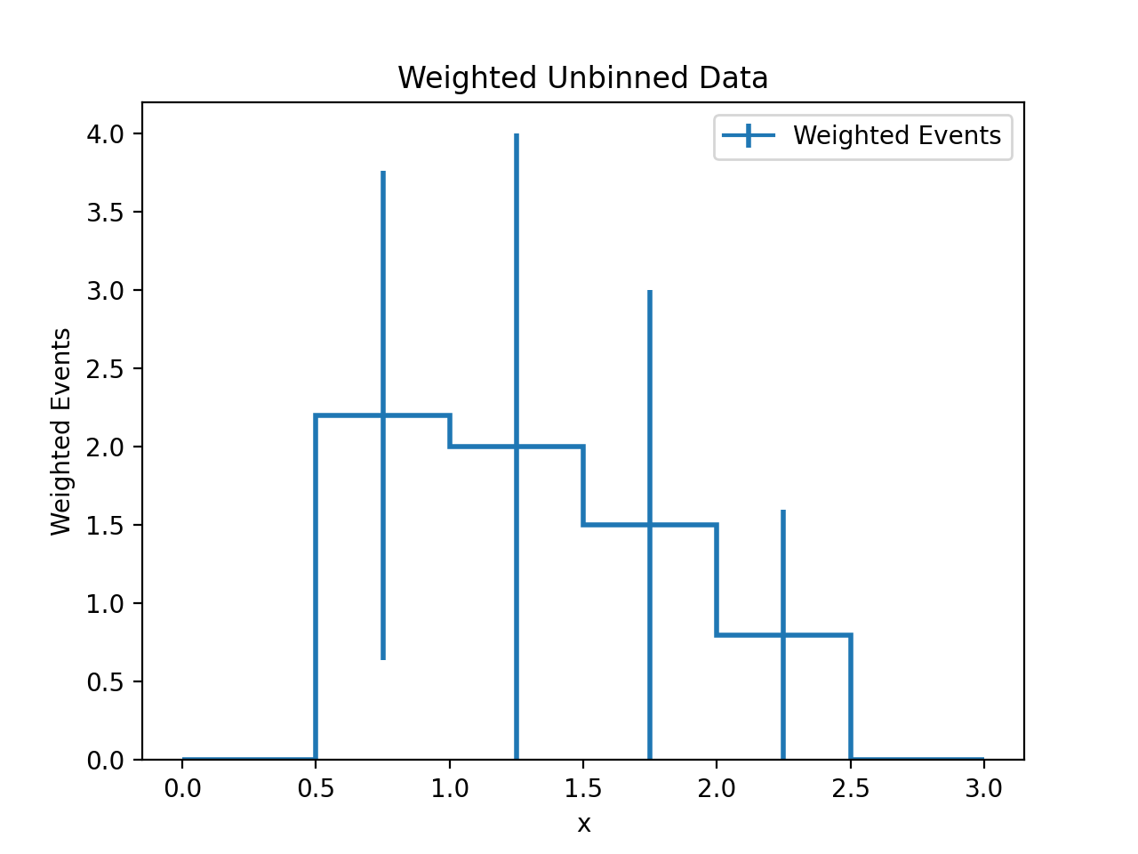
Unbinned Data with Weights
from pyhs3.data import UnbinnedData
from pyhs3.axes import UnbinnedAxis

# Create weighted unbinned data
entries = [[0.5], [1.2], [1.8], [2.3], [0.9]]
weights = [1.0, 2.0, 1.5, 0.8, 1.2]  # Weight for each entry

data = UnbinnedData(
    name="weighted_events",
    type="unbinned",
    entries=entries,
    axes=[UnbinnedAxis(name="x", min=0.0, max=3.0)],
    weights=weights
)

# Convert to hist (weights are applied)
h = data.to_hist(nbins=6)
h.plot(histtype="step", linewidth=2, label="Weighted Events")
plt.xlabel("x")
plt.ylabel("Weighted Events")
plt.legend()
plt.title("Weighted Unbinned Data")
(Source code, png, hires.png, pdf)

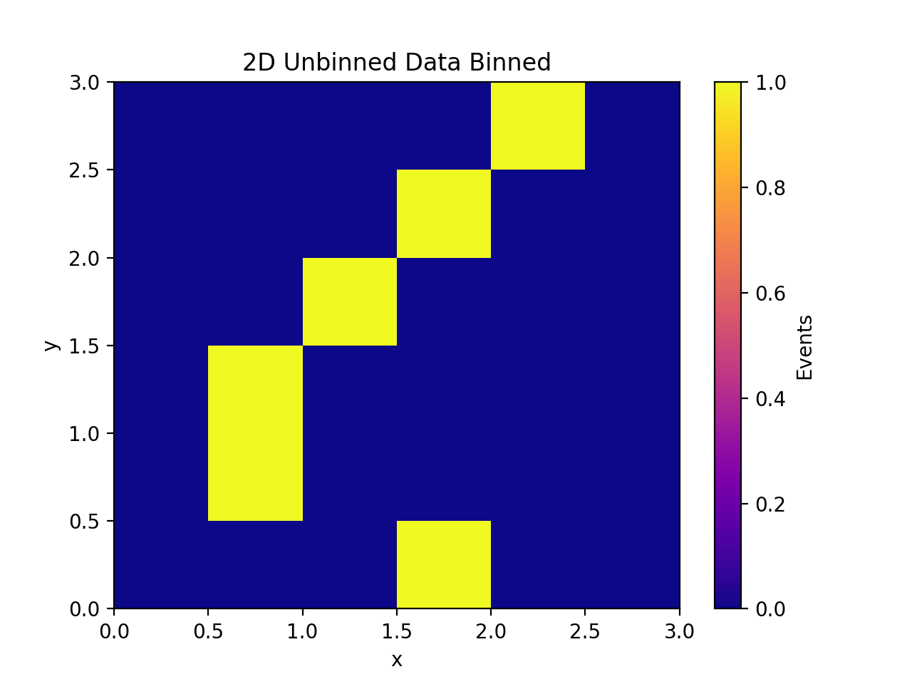
2D Unbinned Data
from pyhs3.data import UnbinnedData
from pyhs3.axes import UnbinnedAxis

# Create 2D unbinned data points
entries = [
    [0.5, 0.8], [1.2, 1.5], [1.8, 0.3],
    [2.3, 2.7], [0.9, 1.2], [1.5, 2.1]
]

data = UnbinnedData(
    name="2d_events",
    type="unbinned",
    entries=entries,
    axes=[
        UnbinnedAxis(name="x", min=0.0, max=3.0),
        UnbinnedAxis(name="y", min=0.0, max=3.0),
    ]
)

# Convert to 2D histogram
h = data.to_hist(nbins=6)
plt.pcolormesh(*h.axes.edges.T, h.values().T, cmap="plasma")
plt.colorbar(label="Events")
plt.xlabel("x")
plt.ylabel("y")
plt.title("2D Unbinned Data Binned")
(Source code, png, hires.png, pdf)

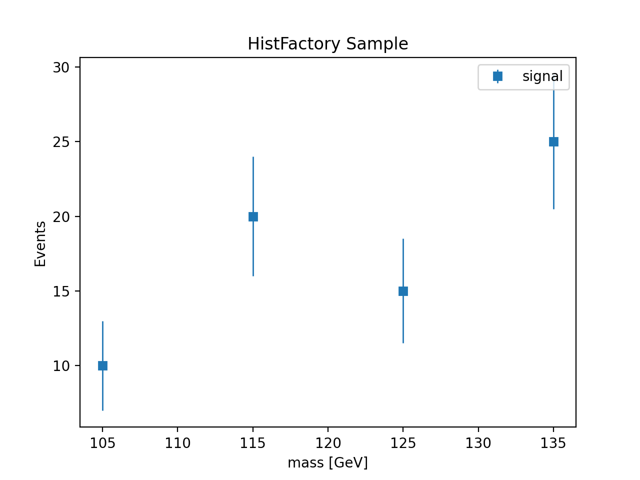
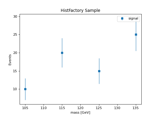
HistFactory Sample to hist
HistFactory Sample objects contain histogram data with statistical errors. The to_hist() method requires an Axes object since the sample itself doesn’t store axis information.
Basic Sample Conversion
from pyhs3.distributions.histfactory.samples import Sample
from pyhs3.axes import Axes

# Create a HistFactory sample
sample = Sample(
    name="signal",
    data={
        "contents": [10.0, 20.0, 15.0, 25.0],
        "errors": [3.0, 4.0, 3.5, 4.5]
    }
)

# Provide axes for binning
axes = Axes([{"name": "mass", "min": 100.0, "max": 140.0, "nbins": 4}])

# Convert to hist
h = sample.to_hist(axes)
h.plot(yerr=True, histtype="errorbar", marker="s", label=sample.name)
plt.xlabel("mass [GeV]")
plt.ylabel("Events")
plt.legend()
plt.title("HistFactory Sample")
(Source code, png, hires.png, pdf)
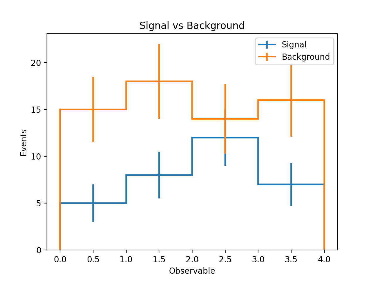
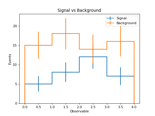
Comparing Multiple Samples
from pyhs3.distributions.histfactory.samples import Sample
from pyhs3.axes import Axes

# Create multiple samples
signal = Sample(
    name="Signal",
    data={"contents": [5.0, 8.0, 12.0, 7.0], "errors": [2.0, 2.5, 3.0, 2.3]}
)

background = Sample(
    name="Background",
    data={"contents": [15.0, 18.0, 14.0, 16.0], "errors": [3.5, 4.0, 3.7, 3.9]}
)

# Common axes for both samples
axes = Axes([{"name": "observable", "min": 0.0, "max": 4.0, "nbins": 4}])

# Convert and plot both
h_signal = signal.to_hist(axes)
h_background = background.to_hist(axes)

h_signal.plot(histtype="step", linewidth=2, label=signal.name)
h_background.plot(histtype="step", linewidth=2, label=background.name)
plt.xlabel("Observable")
plt.ylabel("Events")
plt.legend()
plt.title("Signal vs Background")
(Source code, png, hires.png, pdf)
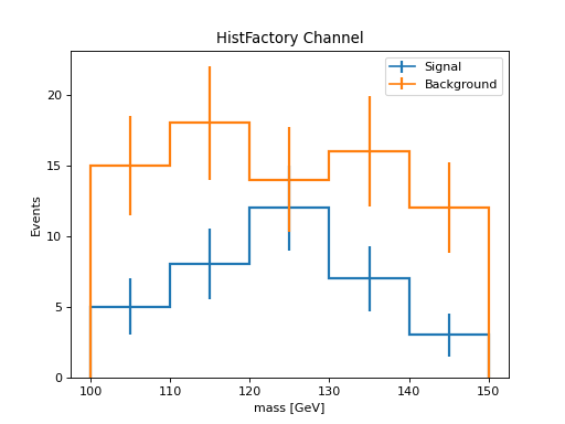
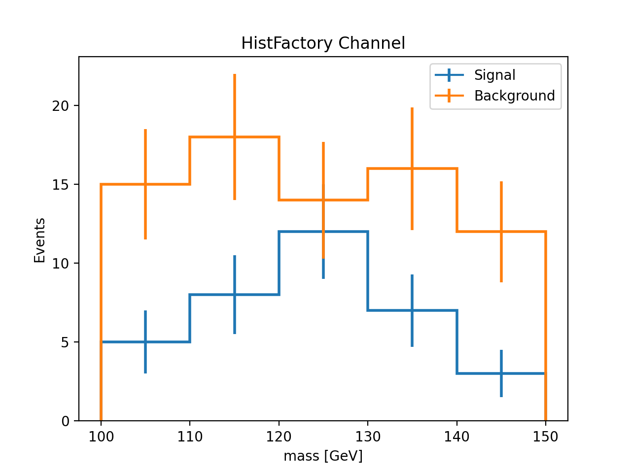
HistFactory Channel to hist
HistFactory HistFactoryDistChannel objects represent complete channels with multiple samples. The to_hist() method creates a single histogram with a categorical “process” axis for distinguishing between samples, followed by the binning axes.
Basic Channel Conversion
from pyhs3.distributions import HistFactoryDistChannel

# Create a HistFactory channel with multiple samples
channel = HistFactoryDistChannel(
    name="SR",
    axes=[{"name": "mass", "min": 100.0, "max": 150.0, "nbins": 5}],
    samples=[
        {
            "name": "signal",
            "data": {"contents": [5.0, 8.0, 12.0, 7.0, 3.0], "errors": [2.0, 2.5, 3.0, 2.3, 1.5]},
            "modifiers": []
        },
        {
            "name": "background",
            "data": {"contents": [15.0, 18.0, 14.0, 16.0, 12.0], "errors": [3.5, 4.0, 3.7, 3.9, 3.2]},
            "modifiers": []
        }
    ]
)

# Convert to hist - creates histogram with categorical "process" axis
h = channel.to_hist()

# Plot both samples from the single histogram
h["signal", :].plot(histtype="step", linewidth=2, label="Signal")
h["background", :].plot(histtype="step", linewidth=2, label="Background")
plt.xlabel("mass [GeV]")
plt.ylabel("Events")
plt.legend()
plt.title("HistFactory Channel")
(Source code, png, hires.png, pdf)

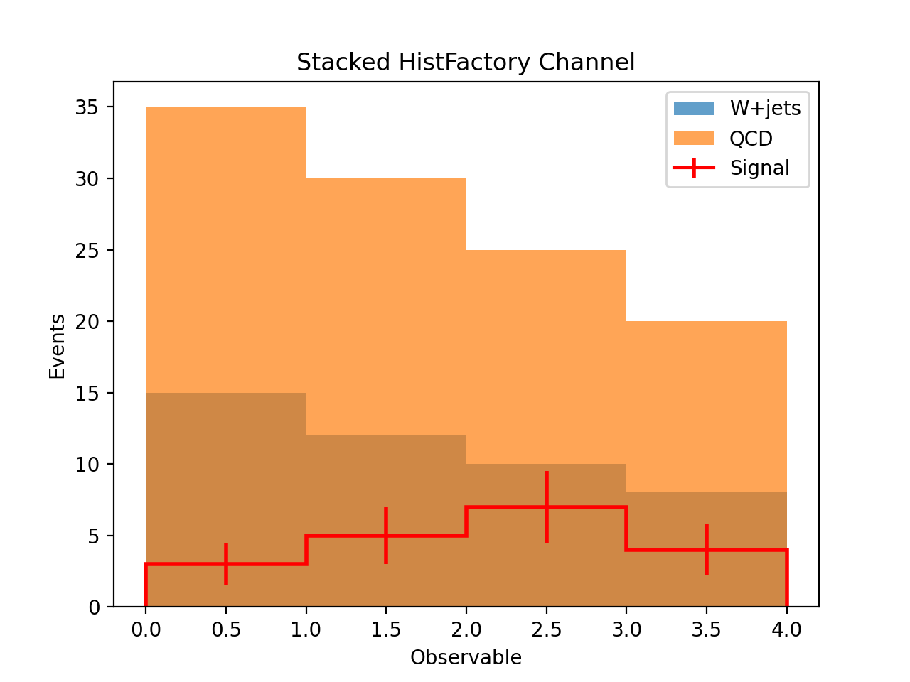
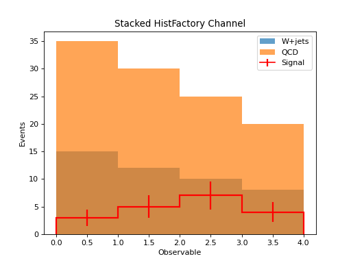
Stacked Histogram from Channel
from pyhs3.distributions import HistFactoryDistChannel

# Create channel with multiple background processes
channel = HistFactoryDistChannel(
    name="channel",
    axes=[{"name": "observable", "min": 0.0, "max": 4.0, "nbins": 4}],
    samples=[
        {
            "name": "Signal",
            "data": {"contents": [3.0, 5.0, 7.0, 4.0], "errors": [1.5, 2.0, 2.5, 1.8]},
            "modifiers": []
        },
        {
            "name": "QCD",
            "data": {"contents": [20.0, 18.0, 15.0, 12.0], "errors": [4.0, 3.8, 3.5, 3.2]},
            "modifiers": []
        },
        {
            "name": "W+jets",
            "data": {"contents": [15.0, 12.0, 10.0, 8.0], "errors": [3.5, 3.2, 3.0, 2.8]},
            "modifiers": []
        }
    ]
)

h = channel.to_hist()

# Create stacked histogram
# Note: hist.stack() requires individual histograms, so we extract them
signal = h["Signal", :]
qcd = h["QCD", :]
wjets = h["W+jets", :]

# Plot stacked backgrounds
plt.stairs(wjets.values(), wjets.axes[0].edges, fill=True, label="W+jets", alpha=0.7)
plt.stairs(wjets.values() + qcd.values(), wjets.axes[0].edges, fill=True, label="QCD", alpha=0.7)

# Overlay signal
signal.plot(histtype="step", linewidth=2, color="red", label="Signal")

plt.xlabel("Observable")
plt.ylabel("Events")
plt.legend()
plt.title("Stacked HistFactory Channel")
(Source code, png, hires.png, pdf)
Customizing Plots
The hist.Hist objects returned by to_hist() support the full matplotlib customization API:
from pyhs3.data import BinnedData
from pyhs3.axes import BinnedAxis

data = BinnedData(
    name="custom",
    type="binned",
    contents=[12.0, 18.0, 15.0, 22.0, 19.0, 14.0],
    axes=[BinnedAxis(name="x", min=0.0, max=6.0, nbins=6)]
)

h = data.to_hist()

# Customize the plot
h.plot(
    histtype="fill",
    alpha=0.5,
    color="steelblue",
    edgecolor="darkblue",
    linewidth=2,
    label="Custom Style"
)

plt.xlabel("Variable", fontsize=14, fontweight="bold")
plt.ylabel("Counts", fontsize=14, fontweight="bold")
plt.title("Customized Histogram", fontsize=16)
plt.grid(True, alpha=0.3, linestyle="--")
plt.legend(fontsize=12)
plt.show()
Working with hist Objects
Once you have a hist.Hist object, you can use all the features of the hist library:
from pyhs3.data import BinnedData
from pyhs3.axes import BinnedAxis

data = BinnedData(
    name="analysis",
    type="binned",
    contents=[10.0, 20.0, 15.0],
    axes=[BinnedAxis(name="x", min=0.0, max=3.0, nbins=3)],
)

h = data.to_hist()

# Access histogram properties
values = h.values()  # Bin contents
edges = h.axes[0].edges  # Bin edges
centers = h.axes[0].centers  # Bin centers

# Statistical operations
total = h.sum()  # Sum of all bins
mean = h.values().mean()  # Mean of bin values

# Rebin the histogram
h_rebinned = h[::2j]  # Rebin by factor of 2

# Save to file
import pickle

with open("histogram.pkl", "wb") as f:
    pickle.dump(h, f)
Limitations
Correlation Matrices Not Preserved
When converting BinnedData with GaussianUncertainty that includes correlation matrices,
only the sigma (standard deviation) values are preserved in the hist.Hist object. The correlation
information is not included because hist does not support correlated uncertainties.
If you need to preserve correlation information, keep the original BinnedData object alongside
the histogram for visualization purposes.